Note: To report bugs with the package, please file an issue on the Github page.
If you use this package, please cite the following:
Kubinec, Robert. “Generalized Ideal Point Models for Time-Varying and Missing-Data Inference”. Working Paper. https://doi.org/10.31219/osf.io/8j2bt.
Note: At present, idealstan uses the cmdstanr package, which is not on CRAN and must be installed separately. Please see below for instructions.
This package implements IRT (item response theory) ideal point models, which are models designed for situations in which actors make strategic choices that correlate with a unidimensional scale, such as the left-right axis in American politics, disagreement over product design in consumer choice, or psychometric scales in which the direction that items load on the latent scale is unknown. Compared to traditional IRT, ideal point models examine the polarizing influence of a set of items on a set of persons, and has similarities to models based on Euclidean latent spaces, such as multi-dimensional scaling. In fact, this package also implements a version of the latent space model for binary outcomes, which is an alternate formulation of an ideal point model.
The goal of idealstan is to offer a wide variety of ideal point models that can model missing-data, time-varying ideal points, and incorporate a range of outcomes, including binary outcomes, counts, continuous and ordinal responses. In addition, idealstan uses the Stan estimation engine to offer full and variational Bayesian inference for all models so that every model is estimated with uncertainty. Variational inference–specifically the Pathfinder algorithm–provides informative starting values to ensure convergence, and for very large models, the possibility of estimating ideal points when full MCMC is impractical. However, the MCMC algorithm has the ability to parallelize within chains using multiple cores, which makes it possible to estimate much larger models with full Bayesian inference than was previously possible.
The approach to handling missing data in this package is to model cases where missing data is a function of a person’s ideal point. In other words, the package will adjust estimates if missingness appears to be correlated with either high or low values of the latent trait. This general missing data adjustment can be usefully applied to many contexts in which a missing outcome is a function of the person’s ideal point (i.e., people will tend to be present in the data when the item is far away or very close to their ideal point). If missingness does not appear to arise as a function of ideal points, the models will still incorporate missing data but will assume it is random conditional on each item.
The package includes the following models:
Table 1: idealstan List of Specifications
Model ID
Model Type
Response Type
Missing Data Adjustment
1
IRT 2-PL
Binary
No
2
IRT 2-PL
Binary
Yes
3
IRT rating scale
Ordinal
No
4
IRT rating scale
Ordinal
Yes
5
IRT graded response
Ordinal
No
6
IRT graded response
Ordinal
Yes
7
IRT 2-PL (Wordfish)
Poisson
No
8
IRT 2-PL (Wordfish)
Poisson
Yes
9
IRT 2-PL
Continuous (Normal)
No
10
IRT 2-PL
Continuous (Normal)
Yes
11
IRT 2-PL
Positive-Continuous (Log-Normal)
No
12
IRT 2-PL
Positive-Continuous (Log-Normal)
Yes
13
Latent Space
Binary
No
14
Latent Space
Binary
Yes
15
IRT 2-PL
Ordered Beta: Proportion (0 to 1 Inclusive)
No
16
IRT 2-PL
Ordered Beta: Proportion (0 to 1 Inclusive)
Yes
In addition, all of these models can be estimated with either time-varying or static ideal points if a column of dates for each item is passed to the model function (see the Time Series vignette). This package implements a range of time series processes (random walk, AR(1), Gaussian processes, and splines). The package also has extensive plotting functions via ggplot2 for model parameters, particularly the legislator (person) ideal points (ability parameters).
This vignette demonstrates how to load data into the package, estimate static ideal points, and also calculate ideal point marginal effects for hierarchical predictors of ideal points.
Installation Instructions
To use idealstan, you first have to have both cmdstanr, an R package, installed and cmdstan, the underlying MCMC library. Unfortunately, cmdstanr is not yet available on CRAN. Simply use the following command to install the package:
# we recommend running this in a fresh R session or restarting your current sessioninstall.packages("cmdstanr", repos =c('https://stan-dev.r-universe.dev', getOption("repos")))
Then you will need to install cmdstan, which is the Stan engine. You can do so by loading cmdstanr and using the function install_cmdstan:
library(cmdstanr)install_cmdstan()
There are some pre-requisites to using cmdstan as you need to be able to compile models on your machine. For example, with Mac OS X you will first need to install Xcode from the Apple App Store. For more details, see complete installation instructions on this page: https://mc-stan.org/cmdstanr/articles/cmdstanr.html.
Assuming you install cmdstan using the functions provided in the package, please allow it to install in the default location.
Simulation of Ordinal IRT with Missing Data
To begin with, we can simulate data from an ordinal ideal-point model in which there are three possible responses corresponding to a legislator voting: yes, abstain and no. An additional category is also simulated that indicates whether a legislator shows up to vote or is absent, which traditional IRT models would record as missing data and would drop from the estimation. This package can instead utilize missing data via a hurdle model in which the censoring of the vote/score data is estimated as a function of individual item/bill intercepts and discrimination parameters for the decision to be absent or present. In other words, if the missing data is a reflection of the person’s ideal point, such as more conservative legislators refusing to show up to vote, than the model will make use of this missing data to infer additional information about the legislators’ ideal points.
The function id_sim_gen() allows you to simulate data from any of the sixteen models currently implemented in idealstan (see previous list). To include missing data, specify the inflate option as TRUE. For example, here we sample data from an ordinal graded response model:
The vote/score matrix in the idealdata object ord_ideal_sim has legislators/persons in the rows and bills/items in the columns. The outcome_disc column has the simulated 3-category ordered outcome.
The function id_estimate will take this processed data and run an IRT ideal point model with the model ID . To specify the model type, either include the model ID from Table 1 as the model_id argument in the id_estimate function or, in the case of multiple models/item types, pass a column model_id to the id_make function that specifies the model ID for each row in the data. This latter option is useful when you have items of mixed types, such as binary, ordinal and/or continuous items. The function id_make also includes the ability to incorporate hierarchical (person or item-level) covariates, as discussed below.
To speed up processing, all of the models shown in Table 1 make use of multiple core parallel computation. To use this option, the specified number of available cores in the ncores option must exceed the number of MCMC chains nchains. cmdstanr will automatically assign cores by dividing the number of chains by the number of cores. In all of the examples in this vignette, I use a machine with 8 cores and estimate 2 chains, so there are 4 cores per chain. By default, id_estimate parallelizes over persons, although that can be changed to items with the map_over_id option (only works with static models).
The package has options for identification that are similar to other IRT packages in which the IDs of legislators/persons to constrain are specified to the id_estimate function. For example, we can use the true values of the simulated legislators to constrain one legislator/person with the highest simulated ideal point and one legislator/person with the lowest ideal point. Each constrained parameter must be fixed to a specific value, preferably at either end of the ideal point spectrum, to identify the model. In particular, two pieces of information are necessary: a value for the high ideal point, and the difference between the high and low points. In this example I pre-specify which parameters to constrain based on the simulated data as restrict_ind_high and restrict_ind_low, and use the actual values to pin the parameters to specific values with fix_high and fix_low.
[1] "Running pathfinder to find starting values"
Path [1] :Initial log joint density = -1440.362379
Path [1] : Iter      log prob        ||dx||      ||grad||     alpha      alpha0      # evals       ELBO    Best ELBO        Notes
             88      -7.324e+02      7.640e-04   8.166e-03    3.837e-01  1.000e+00      2201 -9.133e+02 -9.133e+02
Path [1] :Best Iter: [76] ELBO (-907.095319) evaluations: (2201)
Finished in  0.5 seconds.
[1] "Estimating model with full Stan MCMC sampler."
Running MCMC with 2 parallel chains, with 4 thread(s) per chain...

Chain 1 Iteration:    1 / 2000 [  0%]  (Warmup)
Chain 1 Informational Message: The current Metropolis proposal is about to be rejected because of the following issue:
Chain 1 Exception: Exception: ordered_logistic: Cut-points is not a valid ordered vector. The element at 2 is -192.687, but should be greater than the previous element, -192.687 (in '/Library/Frameworks/R.framework/Versions/4.4-arm64/Resources/library/idealstan/stan_files//chunks/model_types_mm_map_persons.stan', line 378, column 6, included from
Chain 1 '/Library/Frameworks/R.framework/Versions/4.4-arm64/Resources/library/idealstan/stan_files//chunks/map_func.stan', line 408, column 0, included from
Chain 1 '/var/folders/4d/m4b3zyn966d7ctnd4hz4zvfh0000gs/T/RtmpSSVA47/model-dd1a1549e887.stan', line 44, column 0) (in '/var/folders/4d/m4b3zyn966d7ctnd4hz4zvfh0000gs/T/RtmpSSVA47/model-dd1a1549e887.stan', line 639, column 2 to line 745, column 21)
Chain 1 If this warning occurs sporadically, such as for highly constrained variable types like covariance matrices, then the sampler is fine,
Chain 1 but if this warning occurs often then your model may be either severely ill-conditioned or misspecified.
Chain 1
Chain 2 Iteration: 1 / 2000 [ 0%] (Warmup)
Chain 2 Informational Message: The current Metropolis proposal is about to be rejected because of the following issue:
Chain 2 Exception: Exception: ordered_logistic: Cut-points is not a valid ordered vector. The element at 2 is 12.7168, but should be greater than the previous element, 12.7168 (in '/Library/Frameworks/R.framework/Versions/4.4-arm64/Resources/library/idealstan/stan_files//chunks/model_types_mm_map_persons.stan', line 378, column 6, included from
Chain 2 '/Library/Frameworks/R.framework/Versions/4.4-arm64/Resources/library/idealstan/stan_files//chunks/map_func.stan', line 408, column 0, included from
Chain 2 '/var/folders/4d/m4b3zyn966d7ctnd4hz4zvfh0000gs/T/RtmpSSVA47/model-dd1a1549e887.stan', line 44, column 0) (in '/var/folders/4d/m4b3zyn966d7ctnd4hz4zvfh0000gs/T/RtmpSSVA47/model-dd1a1549e887.stan', line 639, column 2 to line 745, column 21)
Chain 2 If this warning occurs sporadically, such as for highly constrained variable types like covariance matrices, then the sampler is fine,
Chain 2 but if this warning occurs often then your model may be either severely ill-conditioned or misspecified.
Chain 2
Chain 2 Informational Message: The current Metropolis proposal is about to be rejected because of the following issue:
Chain 2 Exception: Exception: ordered_logistic: Cut-points is not a valid ordered vector. The element at 2 is -2.34072, but should be greater than the previous element, -2.34072 (in '/Library/Frameworks/R.framework/Versions/4.4-arm64/Resources/library/idealstan/stan_files//chunks/model_types_mm_map_persons.stan', line 378, column 6, included from
Chain 2 '/Library/Frameworks/R.framework/Versions/4.4-arm64/Resources/library/idealstan/stan_files//chunks/map_func.stan', line 408, column 0, included from
Chain 2 '/var/folders/4d/m4b3zyn966d7ctnd4hz4zvfh0000gs/T/RtmpSSVA47/model-dd1a1549e887.stan', line 44, column 0) (in '/var/folders/4d/m4b3zyn966d7ctnd4hz4zvfh0000gs/T/RtmpSSVA47/model-dd1a1549e887.stan', line 639, column 2 to line 745, column 21)
Chain 2 If this warning occurs sporadically, such as for highly constrained variable types like covariance matrices, then the sampler is fine,
Chain 2 but if this warning occurs often then your model may be either severely ill-conditioned or misspecified.
Chain 1 Informational Message: The current Metropolis proposal is about to be rejected because of the following issue:
Chain 1 Exception: Exception: ordered_logistic: Cut-points is not a valid ordered vector. The element at 2 is -3.15566, but should be greater than the previous element, -3.15566 (in '/Library/Frameworks/R.framework/Versions/4.4-arm64/Resources/library/idealstan/stan_files//chunks/model_types_mm_map_persons.stan', line 378, column 6, included from
Chain 1 '/Library/Frameworks/R.framework/Versions/4.4-arm64/Resources/library/idealstan/stan_files//chunks/map_func.stan', line 408, column 0, included from
Chain 1 '/var/folders/4d/m4b3zyn966d7ctnd4hz4zvfh0000gs/T/RtmpSSVA47/model-dd1a1549e887.stan', line 44, column 0) (in '/var/folders/4d/m4b3zyn966d7ctnd4hz4zvfh0000gs/T/RtmpSSVA47/model-dd1a1549e887.stan', line 639, column 2 to line 745, column 21)
Chain 1 If this warning occurs sporadically, such as for highly constrained variable types like covariance matrices, then the sampler is fine,
Chain 1 but if this warning occurs often then your model may be either severely ill-conditioned or misspecified.
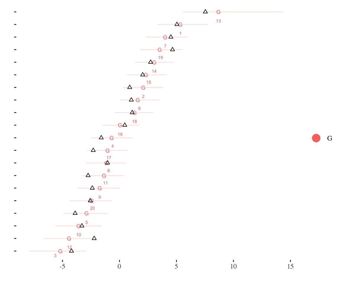
We can then check and see how well the Stan estimation engine was able to capture the “true” values used in the simulation by plotting the true ideal points relative to the estimated ones:
id_plot_legis(ord_ideal_est,show_true =TRUE)
Joining with `by = join_by(id_num)`
Joining with `by = join_by(id_num)`
Given the small amount of data used to estimate the model, the imprecision with which the ideal points were recovered is not surprising. However, the uncertainty intervals generally include the true values, indicating a model that is functioning correctly at recovering estimates even with substantial measurement error.
To automatically identify the model (that is, identify people to fix high or low), simply change the fixtype option to 'vb_full'. By default, the model will select the highest and lowest ideal points to constrain by running an approximation to the full posterior using cmdstanr’s pathfinder() function. While this method works, the exact rotation is not known a priori, and so it may produce a different result with multiple runs. Note that there will be two pathfinder runs as the first run identifies the parameters to constrain and the second is used to create starting values for the Hamiltonian Monte Carlo estimation.
For example, using our simulated data and identifying the model automatically with 'vb_full':
[1] "(First Step): Estimating model with Pathfinder (variational inference) to identify modes to constrain."
Path [1] :Initial log joint density = -2187.233775
Path [1] : Iter      log prob        ||dx||      ||grad||     alpha      alpha0      # evals       ELBO    Best ELBO        Notes
             96      -7.426e+02      8.275e-04   3.336e-03    1.000e+00  1.000e+00      2401 -9.295e+02 -9.295e+02
Path [1] :Best Iter: [91] ELBO (-925.015733) evaluations: (2401)
Finished in  0.5 seconds.
[1] "Running pathfinder to find starting values"
Path [1] :Initial log joint density = -1444.274806
Path [1] : Iter      log prob        ||dx||      ||grad||     alpha      alpha0      # evals       ELBO    Best ELBO        Notes
             85      -7.264e+02      4.887e-04   7.314e-03    5.075e-01  1.000e+00      2126 -9.097e+02 -9.097e+02
Path [1] :Best Iter: [85] ELBO (-909.683971) evaluations: (2126)
Finished in  0.5 seconds.
[1] "Estimating model with full Stan MCMC sampler."
Running MCMC with 2 parallel chains, with 4 thread(s) per chain...

Chain 1 Iteration:    1 / 2000 [  0%]  (Warmup)
Chain 1 Informational Message: The current Metropolis proposal is about to be rejected because of the following issue:
Chain 1 Exception: Exception: ordered_logistic: Cut-points is not a valid ordered vector. The element at 2 is -110.158, but should be greater than the previous element, -110.158 (in '/Library/Frameworks/R.framework/Versions/4.4-arm64/Resources/library/idealstan/stan_files//chunks/model_types_mm_map_persons.stan', line 378, column 6, included from
Chain 1 '/Library/Frameworks/R.framework/Versions/4.4-arm64/Resources/library/idealstan/stan_files//chunks/map_func.stan', line 408, column 0, included from
Chain 1 '/var/folders/4d/m4b3zyn966d7ctnd4hz4zvfh0000gs/T/RtmpSSVA47/model-dd1a1549e887.stan', line 44, column 0) (in '/var/folders/4d/m4b3zyn966d7ctnd4hz4zvfh0000gs/T/RtmpSSVA47/model-dd1a1549e887.stan', line 639, column 2 to line 745, column 21)
Chain 1 If this warning occurs sporadically, such as for highly constrained variable types like covariance matrices, then the sampler is fine,
Chain 1 but if this warning occurs often then your model may be either severely ill-conditioned or misspecified.
Chain 1
Chain 2 Iteration: 1 / 2000 [ 0%] (Warmup)
Chain 2 Informational Message: The current Metropolis proposal is about to be rejected because of the following issue:
Chain 2 Exception: Exception: ordered_logistic: Cut-points is not a valid ordered vector. The element at 2 is -53.5944, but should be greater than the previous element, -53.5944 (in '/Library/Frameworks/R.framework/Versions/4.4-arm64/Resources/library/idealstan/stan_files//chunks/model_types_mm_map_persons.stan', line 378, column 6, included from
Chain 2 '/Library/Frameworks/R.framework/Versions/4.4-arm64/Resources/library/idealstan/stan_files//chunks/map_func.stan', line 408, column 0, included from
Chain 2 '/var/folders/4d/m4b3zyn966d7ctnd4hz4zvfh0000gs/T/RtmpSSVA47/model-dd1a1549e887.stan', line 44, column 0) (in '/var/folders/4d/m4b3zyn966d7ctnd4hz4zvfh0000gs/T/RtmpSSVA47/model-dd1a1549e887.stan', line 639, column 2 to line 745, column 21)
Chain 2 If this warning occurs sporadically, such as for highly constrained variable types like covariance matrices, then the sampler is fine,
Chain 2 but if this warning occurs often then your model may be either severely ill-conditioned or misspecified.
Chain 2
Chain 2 Informational Message: The current Metropolis proposal is about to be rejected because of the following issue:
Chain 2 Exception: Exception: ordered_logistic: Cut-points is not a valid ordered vector. The element at 2 is -8.67553, but should be greater than the previous element, -8.67553 (in '/Library/Frameworks/R.framework/Versions/4.4-arm64/Resources/library/idealstan/stan_files//chunks/model_types_mm_map_persons.stan', line 378, column 6, included from
Chain 2 '/Library/Frameworks/R.framework/Versions/4.4-arm64/Resources/library/idealstan/stan_files//chunks/map_func.stan', line 408, column 0, included from
Chain 2 '/var/folders/4d/m4b3zyn966d7ctnd4hz4zvfh0000gs/T/RtmpSSVA47/model-dd1a1549e887.stan', line 44, column 0) (in '/var/folders/4d/m4b3zyn966d7ctnd4hz4zvfh0000gs/T/RtmpSSVA47/model-dd1a1549e887.stan', line 639, column 2 to line 745, column 21)
Chain 2 If this warning occurs sporadically, such as for highly constrained variable types like covariance matrices, then the sampler is fine,
Chain 2 but if this warning occurs often then your model may be either severely ill-conditioned or misspecified.
Chain 2
Chain 2 Informational Message: The current Metropolis proposal is about to be rejected because of the following issue:
Chain 2 Exception: Exception: ordered_logistic: Cut-points is not a valid ordered vector. The element at 2 is -12.5718, but should be greater than the previous element, -12.5718 (in '/Library/Frameworks/R.framework/Versions/4.4-arm64/Resources/library/idealstan/stan_files//chunks/model_types_mm_map_persons.stan', line 378, column 6, included from
Chain 2 '/Library/Frameworks/R.framework/Versions/4.4-arm64/Resources/library/idealstan/stan_files//chunks/map_func.stan', line 408, column 0, included from
Chain 2 '/var/folders/4d/m4b3zyn966d7ctnd4hz4zvfh0000gs/T/RtmpSSVA47/model-dd1a1549e887.stan', line 44, column 0) (in '/var/folders/4d/m4b3zyn966d7ctnd4hz4zvfh0000gs/T/RtmpSSVA47/model-dd1a1549e887.stan', line 639, column 2 to line 745, column 21)
Chain 2 If this warning occurs sporadically, such as for highly constrained variable types like covariance matrices, then the sampler is fine,
Chain 2 but if this warning occurs often then your model may be either severely ill-conditioned or misspecified.
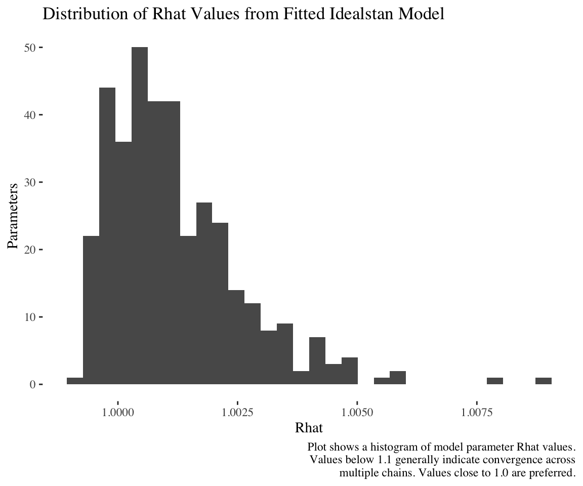
We can see from the plot of the Rhats, which is an MCMC convergence diagnostic, that all the Rhats are below 1.1, which is a good (though not perfect) sign that the model is fully identified:
id_plot_rhats(ord_ideal_est)
`stat_bin()` using `bins = 30`. Pick better value with `binwidth`.
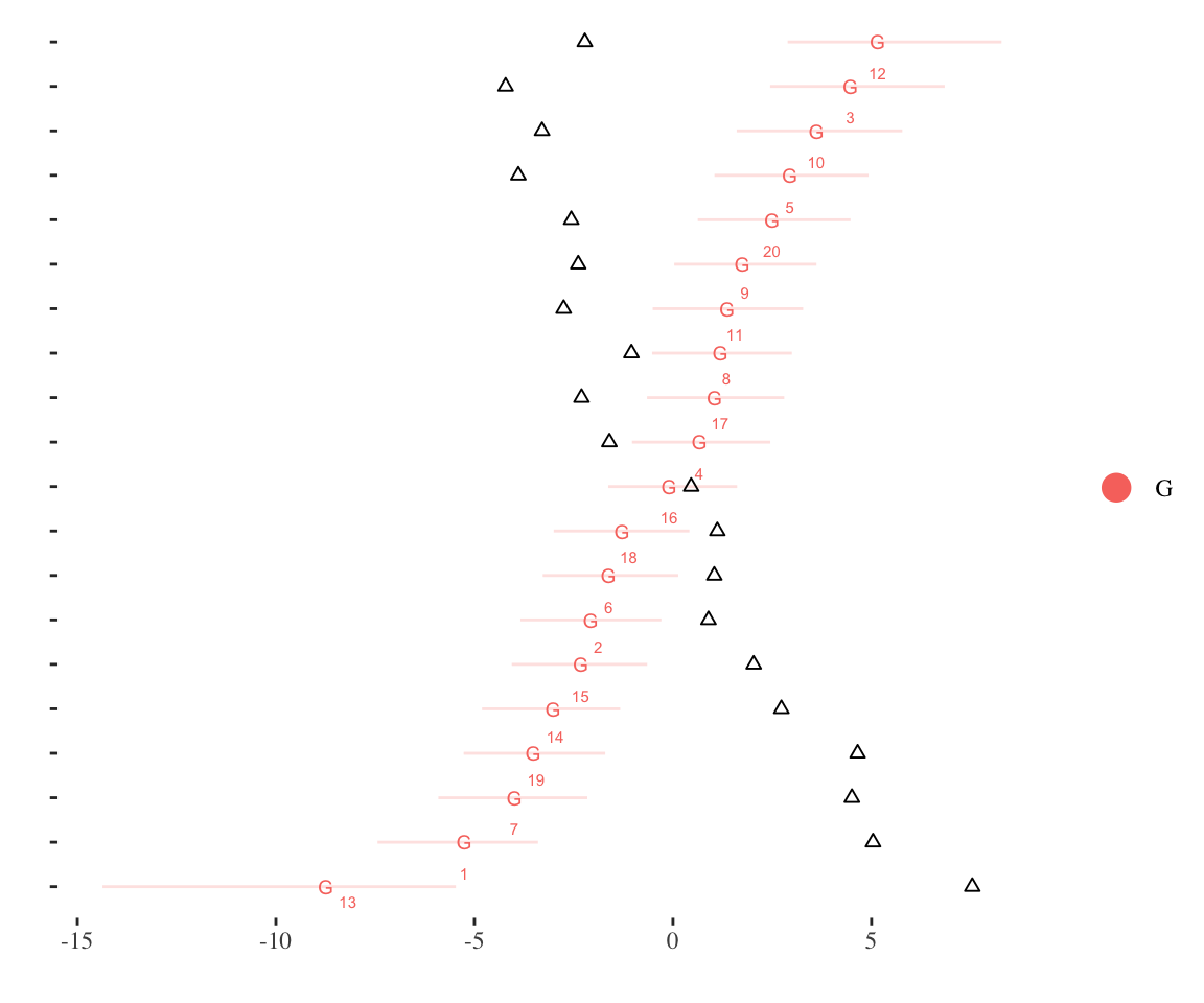
id_plot_legis(ord_ideal_est,show_true = T)
Joining with `by = join_by(id_num)`
Joining with `by = join_by(id_num)`
In general, it is always a good idea to check the Rhats before proceeding with further analysis. Identification of time-varying ideal point models can be more complicated and is discussed in the accompanying vignette. As can be seen above, while the Pathfinder algorithm will usually identify a unique rotation of the ideal points without using any other prior information, it may not be the rotation that is theoretically interesting. For that reason, I recommend specifying persons or items to pin to specific values for applied use of the package as I show in the next section.
Empirical Example: U.S. Senate
This package was developed for datasets that are in a long format, i.e., one row per person/legislator, item/bill, and any other covariates. This data format departs from the traditional way of storing/using IRT/ideal point data, which is more commonly stored in a wide format with legislators/persons in the rows and items/bills in the columns.
To demonstrate how the package functions empirically, I include in the package a partial voting record of the 114th Senate (excluding rollcall votes without significant disagreement) from the website www.voteview.com. We can convert this data, which is provided in a long data frame, to an idealdata object suitable for estimation by using the id_make function. Because the intention is to fit a binary outcome model (yes or no votes on bills), I recode the outcome to be 0 for no votes and 1 for yes votes as idealstan expects binary outcomes to be coded this way.
We can first take a look at the raw data:
data('senate114')tt(select(head(senate114),1:8))
bioname
born
party_code
rollnumber
date
cast_code
congress
chamber
SESSIONS, Jefferson Beauregard III (Jeff)
1946
R
4
2015-01-20
Yes
114
Senate
SESSIONS, Jefferson Beauregard III (Jeff)
1946
R
5
2015-01-20
Yes
114
Senate
SESSIONS, Jefferson Beauregard III (Jeff)
1946
R
7
2015-01-21
Yes
114
Senate
SESSIONS, Jefferson Beauregard III (Jeff)
1946
R
8
2015-01-21
No
114
Senate
SESSIONS, Jefferson Beauregard III (Jeff)
1946
R
9
2015-01-21
Yes
114
Senate
SESSIONS, Jefferson Beauregard III (Jeff)
1946
R
11
2015-01-21
No
114
Senate
table(senate114$cast_code)
    No    Yes Absent
 11233  12119    648
First, you can see that the data are in long form because there is one row for every vote cast by a legislator, in this case Senator Sessions. The outcome variable is cast_code. This variable is coded as a factor variable with the levels in the order we would want for a binary outcome, i.e, 'No' is before 'Yes'. Each item in the model is a recorded vote in the Senate, the numbers of which are listed in column rollnumber. We also know the dates of the individual items (rollcalls), which we will use in the time-varying ideal point vignette to model time-varying ideal points.
The table shows that there are roughly twice as many yes votes versus no votes, with a small minority of absences. In this case, absences can be counted as missing data.
To create an idealdata object for modeling from our long data frame, we pass it to the id_make function and specify the names of the columns that correspond to person IDs, item IDs, group IDs (i.e., party), time IDs and the discrete outcome, although only person, item and outcome are required for the function to work for a static model. Because this is a discrete model, we pass the column name for the outcome to the outcome_disc argument. If we also had items with multiple outcome distributions, we would need to specify the model_id column with the correct model number for each item (see Table 1) and put all continuous (real) data in a separate column which we could pass to the outcome_cont argument.
Note that all missing data should be coded as NA before passing it to id_make.
There are many other columns in the senate114 data. These can be used as person or item/bill covariates, as is discussed at the end of the vignette, but are essentially ignored unless specified to the id_make function.
# set missing (Absent) to NAsenate114$cast_code <-ifelse(senate114$cast_code=="Absent",NA,senate114$cast_code)# recode outcome to 0/1senate114$cast_code <- senate114$cast_code -1senate_data <-id_make(senate114,outcome_disc ='cast_code',person_id ='bioname',item_id ='rollnumber',group_id='party_code',time_id='date')
We can then run a binary IRT ideal point model in which absences on particular bills are treated as a “hurdle” that the legislator must overcome in order to show up to vote. To do so, we specify model_type=2, which signifies a binary IRT model with missing-data (absence) inflation (see list in Table 1). In essence, the model is calculating a separate ideal point position for each bill/item that represents the bill’s importance to different senators. Only if a bill is relatively salient will a legislator choose to show up and vote.
This same missing-data mechanism also applies more broadly to situations of social choice. Any time that missing data might be a function of ideal points–people with certain ideal points are likely to avoid giving an answer–then these values should be marked as NA in the data and an inflated model type should be used. Otherwise, the missing data will be ignored during estimation.
Ideal points are not identified without further information about the latent scale, especially its direction: should conservative ideal points be listed as positive or negative? To identify the latent scale, I constrain a conservative senator (John Barrasso) to be positive, and a liberal senator, Elizabeth Warren, to be negative in order to identify the polarity in the model. I have to pass in the names of the legislators as they exist in the IDs present in the senate114 data (column bionames). The person ideal point parameters are pinned to +1 and -1 but these values can be changed with the fix_high and fix_low function arguments for id_estimate.
It is important to note that the model can also be identified by fixing item (bill) discrimination parameters by setting the const_type argument to "items". Then the values for restrict_ind_high and restrict_ind_low should be set to the character values of names for items in the data. Identifying the model based on item discrimination can have some excellent properties as it leaves all of the person ideal points to float. It is also very useful with time-varying models where fixing person ideal points can be very challenging.
To make the model fit faster, I set nchains at 2 and ncores at 8, which will allow for 4 cores to be used per chain for parallel processing (assuming of course the computer has access to 8 cores).
sen_est <-id_estimate(senate_data,model_type =1,ncores=8,nchains=2,fixtype='prefix',restrict_ind_high ="WARREN, Elizabeth",restrict_ind_low="BARRASSO, John A.",seed=84520)
[1] "Running pathfinder to find starting values"
Finished in  3.1 seconds.
[1] "Estimating model with full Stan MCMC sampler."
Running MCMC with 2 parallel chains, with 4 thread(s) per chain...

Chain 1 finished in 121.7 seconds.
Chain 2 finished in 123.9 seconds.

Both chains finished successfully.
Mean chain execution time: 122.8 seconds.
Total execution time: 124.0 seconds.
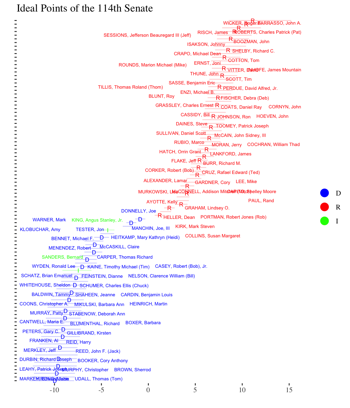
id_plot_legis(sen_est,person_ci_alpha=0.2) +scale_color_manual(values=c(D='blue',R='red',I='green')) +ggtitle('Ideal Points of the 114th Senate')
Joining with `by = join_by(id_num)`
The id_plot function has many other options which are documented in the help files. One notable option, though, is to plot bill midpoints along with the legislator ideal points. The midpoints show the line of equiprobability, i.e., at what ideal point is a legislator with that ideal point indifferent to voting on a bill (or answering an item correctly). To plot a bill midpoint overlay, simply include the character ID of the bill (equivalent to the column name of the bill in the rollcall vote matrix) as the item_plot option:
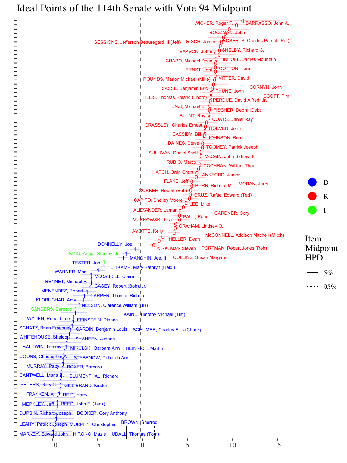
id_plot_legis(sen_est,person_ci_alpha=0.1,item_plot='94') +scale_color_manual(values=c(D='blue',R='red',I='green')) +ggtitle('Ideal Points of the 114th Senate with Vote 94 Midpoint')
Joining with `by = join_by(id_num)`
The 50th bill in the 114 Senate shows very high discrimination: the bill midpoint is right in the middle of the ideal point distribution, with most Democrats voting yes and most Republicans voting no. The two rug lines at the bottom of the plot show the high density posterior interval for the bill midpoint, and as can be seen, the uncertainty only included those legislators near the very center of the distribution.
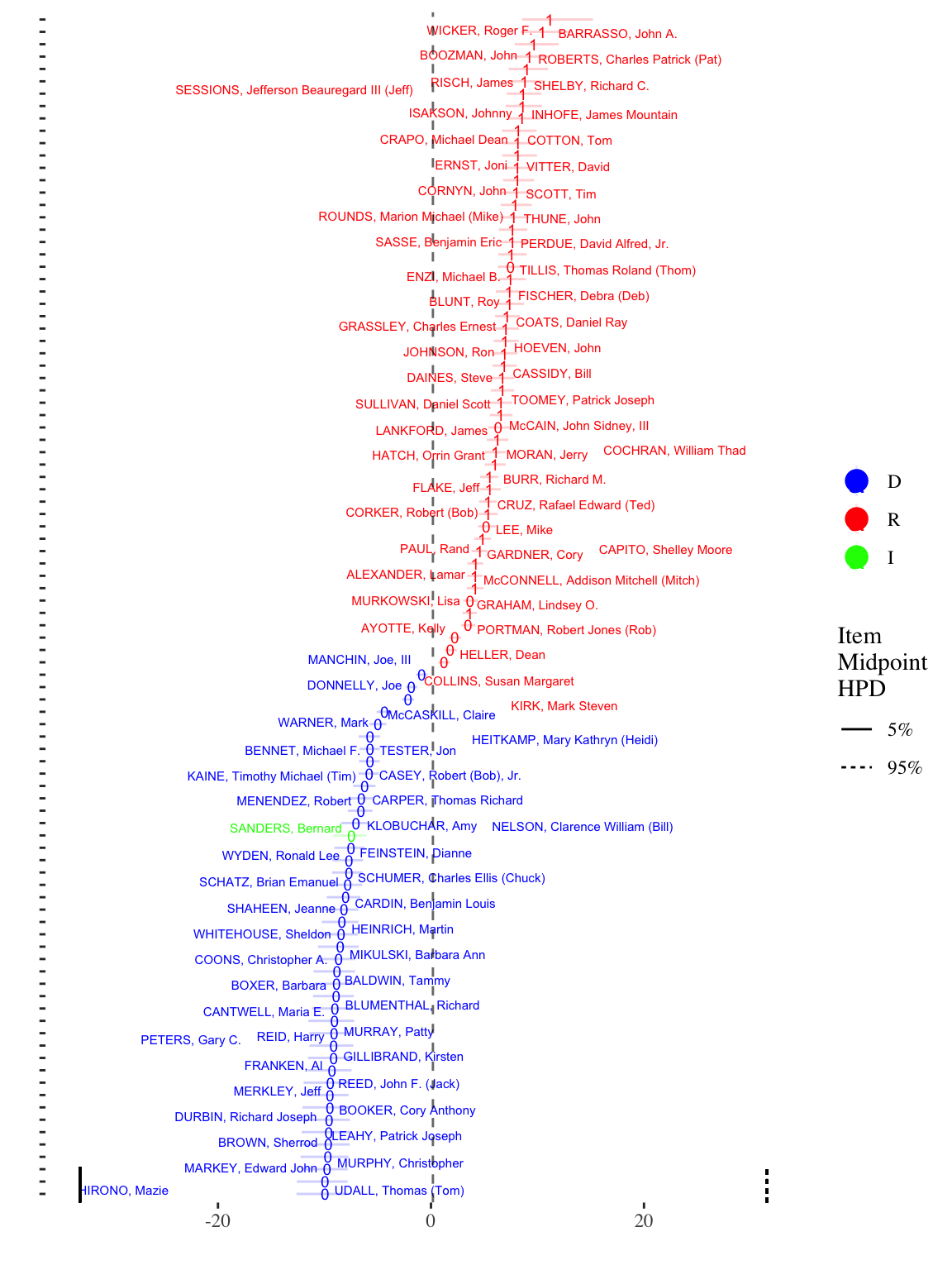
To look at the bill’s absence midpoints, simply change the item_plot_type parameter to the id_plot function:
The wide high-posterior density (HPD) interval of the absence midpoint ruglines shows that absences are very uninformative of ideal points for this particular bill (as is common in the Senate where absences are very rare).
Parameter Values
We can obtain summary estimates of all the ideal points and item/bill discrimination/difficulty parameters using the summary function that provides the median value of the parameters in addition to a specified posterior density interval (i.e., 5%-95%). For example, we can extract summaries for the ideal points:
ideal_pts_sum <-summary(sen_est,pars='ideal_pts')
Joining with `by = join_by(id_num)`
tt(head(ideal_pts_sum))
Person
Group
Time_Point
Low Posterior Interval
Posterior Median
High Posterior Interval
Parameter Name
WYDEN, Ronald Lee
D
1
5.952524
7.220620
8.749867
L_full[100]
BOXER, Barbara
D
1
6.744084
8.446485
10.876780
L_full[10]
BROWN, Sherrod
D
1
7.207698
9.222960
11.785240
L_full[11]
BURR, Richard M.
R
1
-6.626769
-5.643545
-4.815080
L_full[12]
CANTWELL, Maria E.
D
1
6.827412
8.636485
11.207475
L_full[13]
CAPITO, Shelley Moore
R
1
-5.786709
-4.977500
-4.277331
L_full[14]
Parameter Name is the name of the parameter in the underlying Stan code, which can be useful f you want to peruse the fitted Stan model (and can be accessed as given in the code below). The name of the parameters for ideal points in the Stan model is L_full (as seen in the summary from above).
stan_obj <- sen_est@stan_samples# show the stan_obj$draws(c("L_full[1]",'L_full[2]','L_full[3]'))
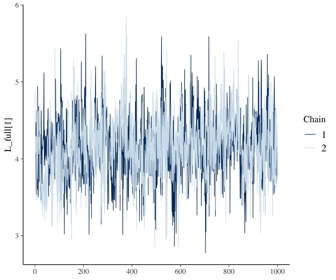
If we know the name of the Stan parameter, we can look at the trace plot to see how the quality of the Markov Chain Monte Carlo (MCMC) sampling used to fit the model. A good trace plot shows a bouncy line that is stable around an average value. For more info, see the Stan documentation.
stan_trace(sen_est,par='L_full[1]')
Finally we can also extract all of the posterior iterations to do additional calculations that average over posterior uncertainty by changing the aggregate option in summary. In the following code, I access the individual posterior iterations for the item/bill parameters, including difficulty (average probability of voting yes), discrimination (how strongly the item/bill loads on either end of the ideal point scale) and the midpoints (position where someone with that ideal point would be indifferent to voting yes/no).
Note: ideal point marginal effects have yet to be implemented as a separate function. In this section I demonstrate how to estimate these effects using R code.
Finally, we can also fit a model where we include a covariate that varies by person/legislator. To do so, we need to pass a one-sided formula to the id_make function to prepare the data accordingly. By way of example, we will include a model where we include an interaction between party ID (party_code) and the legislator’s age to see if younger/older legislators are more or less conservative. Because this is a static model, the effect of the covariate is averaged over all of the bills in the dataset and all the legislators in the dataset without taking into account the order or time period of the bills.
It is important to note that for static ideal point models, covariates are only defined over the legislators/persons who are not being used as constraints in the model, such as John Barasso and Elizabeth Warren in this model.
senate114$age <-2018- senate114$born# center the variablesenate114$age <- senate114$age -mean(senate114$age)# put in units of 10 yearssenate114$age <- senate114$age /10# doing this will improve estimation speed (variables mean-centered and with an SD# not much bigger than 1 or 2)senate_data <-id_make(senate114,outcome_disc ='cast_code',person_id ='bioname',item_id ='rollnumber',group_id='party_code',time_id='date',person_cov =~party_code*age)sen_est_cov <-id_estimate(senate_data,model_type =1,fixtype='prefix',nchains=2,ncores=8,restrict_ind_high ="BARRASSO, John A.",restrict_ind_low="WARREN, Elizabeth",seed=84520)
[1] "Running pathfinder to find starting values"
Finished in  5.6 seconds.
[1] "Estimating model with full Stan MCMC sampler."
Running MCMC with 2 parallel chains, with 4 thread(s) per chain...

Chain 1 finished in 240.1 seconds.
Chain 2 finished in 240.2 seconds.

Both chains finished successfully.
Mean chain execution time: 240.2 seconds.
Total execution time: 240.4 seconds.
As discussed in the associated working paper (https://osf.io/preprints/osf/8j2bt), ideal point marginal effects can be derived from idealstan models in which the raw relationship between the hierarchical covariates and the actual outcomes (in this case, votes) can be shown at the item (vote) level. There are two functions that can be used to calculate and display ideal point marginal effects. The first, id_me, shown in the chunks, below, will produce data frames with summaries ideal point marginal effects given a covariate and also data frames with one row per posterior draw that are useful for further analysis or aggregation.
In the example below, ideal point marginal effects are calculated for the "age" covariate, first for the whole dataset and then for all distinct values of "group_id", which is party ID in our data. This latter calculation is especially useful as we interaction age with group_id, and by calculating marginal effects for each distinct subset of group_id we can learn what the conditional marginal effect is by party ID.
# calculate marginal effects for age subset by item marg_effs <-id_me(sen_est_cov,covariate="age")
Creating predictions
[1] "Processing posterior replications for 23352 scores using 100 posterior samples out of a total of 2000 samples."
[1] "Adding in hierarchical covariates values to the time-varying person scores."
[1] "Collapsing covariates to person and time IDs."
[1] "Done!"
[1] "Now on model 1"
[1] "Processing posterior replications for 23352 scores using 100 posterior samples out of a total of 2000 samples."
[1] "Adding in hierarchical covariates values to the time-varying person scores."
[1] "Collapsing covariates to person and time IDs."
[1] "Done!"
[1] "Now on model 1"
Differencing
Joining with `by = join_by(item_id)`
  head(marg_effs$ideal_effects) %>%
    tt
draws
item_id
person_id
estimate
group_id
item_orig
person_orig
model_id
1
1
1
0.0010801271
R
4
ALEXANDER, Lamar
1
2
1
1
0.0004783580
R
4
ALEXANDER, Lamar
1
3
1
1
0.0014135599
R
4
ALEXANDER, Lamar
1
4
1
1
0.0004605616
R
4
ALEXANDER, Lamar
1
5
1
1
0.0054023860
R
4
ALEXANDER, Lamar
1
6
1
1
0.0017234928
R
4
ALEXANDER, Lamar
1
  head(marg_effs$sum_ideal_effects) %>%
    tt
item_id
item_orig
model_id
mean_est
low_est
high_est
item_discrimination
1
4
1
-0.020532272
-0.136937626
0.004289538
0.6749270
2
5
1
-0.002767829
-0.043591668
0.035765552
0.5672335
3
7
1
-0.005987748
-0.036915911
0.014117922
0.7255410
4
8
1
0.024729912
-0.006075327
0.155946659
-0.5813605
5
9
1
-0.007212386
-0.069622873
0.032293252
0.4334265
6
11
1
-0.019462043
-0.085609055
0.018203017
-0.3371580
# now group marginal effects by group_id (party ID) marg_effs_grouped <-id_me(sen_est_cov,covariate="age",group_effects="group_id")
Creating predictions
[1] "Processing posterior replications for 23352 scores using 100 posterior samples out of a total of 2000 samples."
[1] "Adding in hierarchical covariates values to the time-varying person scores."
[1] "Collapsing covariates to person and time IDs."
[1] "Done!"
[1] "Now on model 1"
[1] "Processing posterior replications for 23352 scores using 100 posterior samples out of a total of 2000 samples."
[1] "Adding in hierarchical covariates values to the time-varying person scores."
[1] "Collapsing covariates to person and time IDs."
[1] "Done!"
[1] "Now on model 1"
In addition to the data frames of the results, the id_plot_cov can take the same arguments, calculate the ideal point marginal effects and then plot them. If we pass a grouping variable, the id_plot_cov function will plot marginal effects in distinct facets for each level of the grouping variable. If there are multiple model ID types, the function will produce distinct facets for each model ID type (note that only one kind of facetting can be used for a given plot).
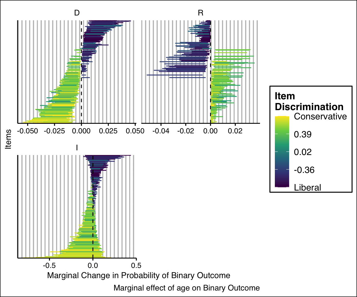
# plot the result sen_est_cov %>%id_plot_cov(calc_param="age",group_effects="group_id",label_high="Conservative",label_low="Liberal")
Creating predictions
[1] "Processing posterior replications for 23352 scores using 100 posterior samples out of a total of 2000 samples."
[1] "Adding in hierarchical covariates values to the time-varying person scores."
[1] "Collapsing covariates to person and time IDs."
[1] "Done!"
[1] "Now on model 1"
[1] "Processing posterior replications for 23352 scores using 100 posterior samples out of a total of 2000 samples."
[1] "Adding in hierarchical covariates values to the time-varying person scores."
[1] "Collapsing covariates to person and time IDs."
[1] "Done!"
[1] "Now on model 1"
Differencing
Grouping marginal effect summaries by group_id
Joining with `by = join_by(item_id)`
Because these covariates are on the ideal point scale, the meaning of the scale in terms of party ideology must be kept in mind in order to interpret the plot. The way to interpret these plots is that older Democrats tend to be more likely to vote for conservative bills, while younger Democrats vote more for liberal bills. The relationship does not hold true for Republicans, who are roughly equally as likely to vote for liberal or conservative bills regardless of age. Keeping the direction of the scale in mind–which is shown on the plot as the colour of the item discrimination for each vote–is crucial for understanding hierarchical covariates in ideal point models.
We can also extract the covariate summary values using the summary function: